Machine learning for IRB model
De laatste paar jaar is er een enorme groei in zowel onderzoek als gebruik naar en van Machine Learning. Ook binnen de financiële sector wordt de technologie meer en meer gebruikt. Binnen het kredietrisico domein heeft de regelgever een paper gepubliceerd met als doel om inzicht te verkrijgen in uitdagingen voor gebruik van Machine Learning voor kwantitatieve modellen volgens Europese banken. In dit paper wordt duidelijk dat ondanks de voordelen die Machine Learning met zich meebrengt er eerst zorgvuldig beoordeeld dient te worden of deze voordelen opwegen tegen de additionele uitdagingen en bijkomende kosten.
Key Messages
With the publication of its discussion paper, EBA has opened the door towards the use of Machine Learning techniques within IRB models;
- Machine Learning techniques are expected to improve risk differentiation significantly, in particular ensemble learners show promising results;
- Use of Machine Learning models within the Internal Ratings Based context requires a fundamental change in among others model governance and training of stakeholders;
- A key success factor is experience with use of Machine Learning;
- Investing in sound Machine Learning model governance, data foundation and training of stakeholders are no regret investments
Background
Last year, the European Banking Authority (EBA) and the European Commission (EC) published two papers both concerning the usage of Artificial Intelligence (AI) and Machine Learning (ML). The EBA discussion paper, published in November 2021, focuses on ML being applied to Internal Ratings Based (IRB) models [7]. The proposal for regulations published in June 2021 by the EC concerned draft regulations of the use of Artificial Intelligence (AI) and Machine Learning (ML) within Europe across all
sectors [8].
These publications are seen as big steps towards regulating the use of AI and ML. Up until then both EBA and local authorities published reports containing best practices, challenges and recommendations concerning usage of AI and ML [6] and [3].
The EBA observed that most ML applications within credit risk do not involve regulatory models. Instead various ML techniques are being used for other credit risk models such as: credit decisions, monitoring and restructuring [7]. For IRB models, the EBA states that due to regulatory requirements direct use of ML is currently avoided. It is only used to complement standard techniques in the following ways:
- Model validation by developing challenger models;
- Data improvements by means of data preparation and data exploration;
- Variable selection to detect suitable explanatory variables; and
- Risk differentiation where a challenger model is used to assess potentially improved risk drivers.
In order for the EBA to gain better insights, the discussion paper comes along with a questionnaire covering: in what areas of IRB modelling institutions are currently using, or planning to use, ML; what methods/algorithms they are planning to use and what challenges institutions expect to face (and cope with) in terms of model development, model governance, model implementation and model documentation. The due date of sending responses to the EBA was February 11th 2022.
Recent academic literature demonstrates that ML algorithms can yield material improvements to risk parameter estimates. We therefore applaud the initiative of the EBA to investigate the potential use of ML within IRB. The purpose of this paper is to discuss some key aspects that financial institutions should consider during their assessment whether or not to adopt ML. Aspects such as training of stakeholders (management, validation and audit) and choice of appropriate ML algorithm can result in substantial additional costs which may hamper the benefits of ML implementation.
This paper starts with an overview of the ML landscape providing background on the different ML algorithms and how they relate to one another in terms of complexity and transparency. The purpose of this is to better understand the second section where we provide an overview of recent academic publications concerning ML algorithms applied to IRB. Most of the cited articles performed comparative analyses on different algorithms. Finally, the challenges stated by the EBA discussion paper are presented which are complemented by our view on certain key points demonstrating the additional complexity that comes with ML adaptation.
High level overview of the Machine Learning Landscape
This section provides a high level overview of the Machine Learning landscape, covering different learning paradigms and discussing common ML algorithms. It serves as a background for the next section which discusses recent academic literature concerning implementation of ML for IRB. The authors of academic publications evaluated a broad range of ML algorithms.
Machine Learning algorithms have their own characteristics, benefits and drawbacks which lead to different purposes. Within the literature, algorithms are categorized into supervised learning, unsupervised learning and reinforcement learning. The EBA discussion paper defines these learning paradigms as:
- Supervised learning (or learning with labels): the algorithm learns rules for building the model from a labelled dataset and uses these rules to predict labels on new input data.
- Unsupervised learning (or learning without labels): the algorithm learns from an input training dataset which has no labels. The goal is to understand the distribution of the data and/or to find a more efficient representation of it.
- Reinforcement learning (or learning by feedback): the algorithm learns from interacting with the environment, rather than from a training dataset. Moreover, contrary to supervised learning, reinforcement learning does not require labelled input/output pairs. The algorithm learns to perform a specific task by trial and error.
For IRB modelling the most prevalent learning paradigm in research is either supervised learning or unsupervised learning. Supervised learning could, among others, be used for risk quantification where the output variable such as default/non-default is known. An example for unsupervised learning is risk differentiation where clustering techniques are used to assign obligors with certain similar characteristics to the same cluster (rating grade).
Given the broad set of potential ML algorithms, choosing the (most) appropriate algorithm becomes more and more important. To help institutions in adopting ML within finance Hoang & Wiegratzn [9] performed a comprehensive analysis where they evaluated multiple supervised and unsupervised ML algorithms in terms of their characteristics, benefits and drawbacks. Given their analyses, commonly used supervised ML algorithms can be schematically presented as follows
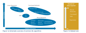
Though Figure 1a does not contain all ML algorithms currently available, it does show a clear trade-off between model performance and interpretability. Additionally Figure 1b shows that for more complex algorithms, a larger amount of data is needed in order to ensure reliable results. This trade-off is dependent on the type of ML application and the regulator’s imposed requirements. The proposal for regulations published by the European Commission [8] subjects high risk applications (e.g. ML based credit scoring) to stricter requirements than low risk applications. Additionally, the EBA discussion paper states various challenges(1) that have to be accounted for when adopting ML for IRB of which interpretability, transparency and explainability are important topics. Management of financial institutions will therefore have to carefully assess which ML algorithm provides good balance between performance and complexity.
As said, the next section discusses recent (academic) publications concerning ML being applied to IRB. We therefore provide a brief introductory explanation for the more commonly used ML algorithms.
Logistic Regression
This model is currently market practice for PD estimation and is a binary classification problem (defaults and non-defaults). It consists of two parts, first log odds are calculated using a linear regression model where various independent variables are regressed on a dependent output variable (default flag). The log odds are a ratio of probability of default to probability of non-default. It represents how much more likely it is to observe a default than a non-default for a certain dataset. The log odds are finally transformed in a probability(2)
Decision Tree
This is a relatively straightforward algorithm where data is split in nodes using business rules (branches). The splits are determined by using impurity scores (e.g. Gini, Entropy or MSE) that assess the quality of the split, i.e. how well the data is segregated. The nodes resulting from the final splits are referred to as leaf nodes. These leaf nodes contain the model’s prediction which is the average of the observed values of the training data.
Though a decision tree is relatively simple and provides easy interpretability, it is an unstable algorithm since a small perturbation of the training data can result in a completely different decision tree. Therefore tree-based ensemble learners have been developed of which the most popular algorithms are Random Forest and Gradient Boosting.
Random Forest
A random forest is a form of ensemble learning, which consists of multiple decision trees. Given the training dataset, multiple random sub-samples are generated using bootstrapping from the original dataset and for each bootstrapped sample a decision tree is built. Each decision tree selects a number of random variables from the full list of variables available in the bootstrapped sample and then creates its branches and (leaf) nodes similarly to a standard decision tree.
Afterwards, when the specified number of decision trees is constructed, the predictions of the individual trees are aggregated (bagging) to get the final prediction of the random forest. In most cases bagging is taking the average prediction.
Gradient Boosting
Gradient Boosting is an ensemble learner where multiple decision trees are constructed. At first a decision tree is constructed as discussed before and then additional (simpler) trees are constructed where each additional tree focuses on the misclassifications (or high error instances) of the previous tree. Building the additional trees is called boosting. There are optimized versions of gradient boosting, examples are XGBoost and Light GBM.
Artificial Neural Networks
A neural network is a form of deep learning where the learning algorithm is based on the human brain. The standard model consists of an input layer, multiple hidden layers and an output layer. Each layer contains neurons that, based on the input data (input layer), pass information along to connected neurons in the next layer. Each neuron can focus on specific aspects of the input data in order to
determine the output which is returned in the output layer.

A schematic overview of a neural network for binary classification is shown in Figure 2. Note that in this simple example the input dataset contains three independent variables and the output layer returns two probabilities, one for each possible label which could be default or non-default.
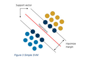
Support Vector Machine
A support vector machine (SVM) fits a hyperplane that for classification differentiates data points and for regression fits most data points. The hyperplane is determined using support vectors which are the data points closest to the hyperplane. The hyperplane is fitted by optimizing the margins between the hyperplane and support vectors. A simple example of SVM for classification is presented in Figure 3 where the two support vectors (dark blue data points) are set such that the margin between the two is maximized. The hyperplane is in the middle of the two support vectors. All data points on the same side of the hyperplane receive the same classification like default or non-default. The algorithm can be used both for regression (i.e. support vector regression, SVR) and classification (i.e. support vector classification, SVC).
Recent Academic Literature on ML for IRB models
This section outlines recent publications demonstrating that ML can be used to either directly estimate the IRB risk parameter or as a supportive function to improve performance of traditional models (i.e. logistic regression). It focuses on ML being applied to either PD or LGD modelling since this is the scope of the majority of academic literature and publications concerning ML being applied to EAD modelling are scarce. It will become clear that the majority of cited publications conclude that ensemble ML algorithms (random forest and gradient boosting) yield the best performance.
Probability of Default
Estimating the PD starts with preparing a reference dataset (RDS) that contains obligor characteristics, financial information and behavioural information. Based on the RDS, exposures with similar characteristics are assigned to the same rating grade (risk differentiation) after which, for each rating grade a PD is calculated (risk quantification). Though the standard technique used for PD estimation is logistic regression, there is a vast amount of literature focusing on more complex ML algorithms being applied to PD estimation, credit scoring or credit decisioning.
Addo, Guegan, & Hassani [1] who perform a comparative analysis on different ML algorithms (logistic regression, random forest, gradient boosting and multiple artificial neural networks) applied to predict defaults in a loan portfolio. The results showed that the ensemble learners, random forest and gradient boosting performed not only best, but also yielded most stable results. Additionally, it is observed that logistic regression selects global and aggregated financial variables while ensemble learners select detailed financial variables.
The Bank of International Settlements (BIS) published a report prepared by the Bank of Greece concerning estimation of the Trough-The-Cycle (TTC) PD for a large dataset of corporate Greek loans [11]. They compared the performance of logistic regression, XGBoost and an artificial neural network on a 3-year out-of-time sample period. Prior to developing the models, they incorporated dimension reduction techniques since the raw dataset contained 354 predictor variables (consisting of macro variables and economic ratios). They used a random forest that classifies variables as either “important” or “noise” (i.e. the Boruta algorithm) and reduced the number of variables to 65. The different models were evaluated in terms of discriminatory power (i.e. Kolmogorov Smirnov and AUC) and in terms of predictability (i.e. Sum Square Errors and Brier score). The results showed that XGBoost performed best for all metrics.
Finally, Dumitrescu et al. [4] developed a workaround given the current trade-off between ML complexity and ML explainability. They introduced the penalised logistic tree regression (PLTR) which utilized information from decision trees to improve the performance of logistic regression for credit scoring. The PLTR model showed a significant improvement over the logistic regression which was comparable with that of a random forest.
Loss Given Default
The estimation process for LGD is more complex than PD estimation since (realized) LGD is usually calculated based on multiple parameters that have to be calculated/estimated separately. In the general case the LGD parameter is not estimated directly but instead parameters like: Probability of Cure (PC), Loss Given Cure (LGC), Loss Given Loss (LGL), Collateral value (e.g. residential real estate(3)), Future recoveries (and expected recovery period) and Future (material) costs (direct and indirect) are estimated and then used to calculate (realized) LGD.
Machine Learning can be applied to estimate certain parameters separately as is shown in literature. For example Xiao, Crook, & Andreeva [13] performed a two-stage model to predict recovery rates, where a classification step was performed to discriminate exposures with recovery rates equal to either 0 and 1. A regression step was performed to estimate recovery rates between 0 and 1. For the classification step, a support vector classifier (SVC) was compared with logistic regression where the authors concluded that the SVC was the preferred technique. For the regression step, multiple regressions were compared with support vector regression (SVR) where authors concluded that the SVR yielded modest improvements. However, on the whole sample the SVR did not present any advantages compared to standard regressions. A comparable study on five Japanese banks was performed by Tanoue & Yamashita [12] where the classification step was replaced by boosted trees and the authors concluded that the boosting method improves the predictive performance.
A third article published by Bellotti et al. [2] assessed forecasting recovery rates for retail Non Performing Loans (mortgages and credit cards) using around twenty different models ranging from linear to nonlinear to ensemble learners. Of these models, the ensemble learners (i.e. random forest, gradient boosting and cubist) yielded the best forecasting performance.
There are also numerous publications on ML being applied to valuing residential properties. Take for example Masias, et al. [10] who performed a comparative study to estimate the residential house prices in Chile. The used models were neural network, random forest, SVM and traditional approaches like regression. The results showed that the random forest model performed better than the other models in terms of root mean squared error, ?2, and mean absolute error. Another study performed by Yazdani [14] on residential property prices in Boulder, Colorado where a traditional model (i.e. hedonic pricing) was compared with Neural Network, Random Forest and K-nearest neighbours. It became clear that both Random Forest and Neural Network outperformed the traditional hedonic regression model.
Considerations on the use of ML for IRB models
The previous section demonstrated that there is a broad set of possibilities to use ML within the IRB space. The literature showed that it can yield better model performance and/or utilize information from unstructured data. This is also recognized by the EBA discussion paper where potential benefits are outlined for different steps in the risk parameter estimation process (data, risk differentiation, risk quantification etc.). The focus of the paper is however on the challenges and specifically how financial institutions (expect to) cope with these when they (opt to) implement ML for IRB. The table below summarizes the (main) challenges posed by the EBA:

Considering these challenges it becomes apparent that quite some additional effort is required by financial institutions if they want to adopt ML for IRB purposes. In the paragraphs below we discuss, what are in our view, important but non-exhaustive aspects that need to be considered as well.
ML model use
One of the most costly processes of ML implementation is training relevant stakeholders such that they are able to work with and understand the models and their output. Note that stakeholders do not only cover developers and management but also validators and auditors. All require sufficient understanding to be able to perform appropriate validations/audits. Additionally, validation policies/standards have to be developed specifically tailored to ML models outlining what tests and procedures need to be performed. Standard procedure for IRB models is to assess discriminatory power, predictive ability etc., but for ML models aspects such as transparency, explainability and latent bias will also have to be addressed.
High versus Low default portfolios
Institutions should carefully assess for which portfolio they want to adopt ML. It is generally known that credit risk modelling can be differentiated between high default portfolios and low default portfolios. The archetype high default portfolios (HDP) are retail and SME portfolios while the large corporate portfolios are often determined to be low default portfolios (LDP). These portfolios have different characteristics and the main differences are in the amount of data available and the complexity of credit structures. While ML might be easier implemented for HDPs, it could yield more significant improvements to implement ML for LDPs.
Choice of the ML model
As shown in the ML landscape paragraph, there is a broad set of ML models, each with their own characteristics. This imposes a challenge for financial institutions to choose the most appropriate ML model for IRB estimation (PD, LGD etc) while taking into account the trade-off between performance and complexity (figure 1a). Currently, logistic regression and decision trees are already used but shifting to more complex models will require additional effort to ensure model transparency, interpretability and explainability. This might also be reflected in more comprehensive validation standards.
Although the Recent Literature paragraph demonstrated that ensemble learners (random forest and gradient boosting) yield the best performance, figure 1b showed that they require larger historic datasets to ensure reliable estimation. Therefore, more resources should be allocated to data collection, data preparation and data quality assessment. If financial institutions have difficulties gathering high quality historical data than it is not advised to switch to more complex ML algorithms but instead stick with simpler algorithms like logistic regression.
Retraining of the ML model
Another key aspect of ML models is that they have to be retrained with a certain frequency. Since some ML algorithms are more prone to overfitting than others (i.e. gradient boosting), their retraining frequency might differ. Therefore, institutions have to carefully assess how frequent the ML model for IRB is retrained. Retraining the model too frequently imposes the risk of deviating from the Long Run Average (LRA) since the difference between consecutive training periods becomes less significant while the overall difference for example between one or two years could yield significant differences.
Variability of IRB estimates
The last couple of years, financial institutions have been involved with adjusting and/or redeveloping their IRB models as part of IRB repair programme. This is an extensive multi-year endeavour during which banks had to incur considerable costs. The purpose of the IRB repair program was to reduce variability in IRB estimates across European financial institutions by publishing among others guidelines and regulatory technical standards (i.e. Guidelines on estimation of PD and LGD (EBA, 2017)).
Since various ML models will by default yield different outcomes, the EBA has to carefully assess how it will ensure comparable estimation results between financial institutions within the European Union. It can therefore be expected that incorporating more complex ML algorithms in the IRB estimation process (differentiation and/or calibration) will initiate a new multi-year program. As a result additional effort is required in order for the ML models to be compliant and again reduce variability.
Conclusion
Adopting ML can yield material benefits for different aspects/components within the IRB space. We observed that ensemble learners yielded the best performance when applied to estimating various risk components within IRB. However, as outlined in the EBA discussion paper, there are also a lot of challenges that need to be taken into account if a financial institution considers to adopt ML for its risk type estimation. Some of these challenges require quite some effort to be resolved and financial institutions should therefore carefully assess whether a ML implementation is worth the additional costs.
We applaud the initiative of the EBA to investigate the potential use of ML within IRB. We also agree with the opinion of the EBA concerning the complexity for financial institutions to be able to implement sound ML models for direct IRB estimation.
- Refer to table 1 for a list of challenges stated by the EBA discussion paper
- For binary classification problems this is done using the sigmoid function

- The EBA Guidelines on Loan Origination and Monitoring allow institutions to support internal/external
desktop valuation with advanced statistical models

References
1. Addo, P., Guegan, D., & Hassani, B. (2018, April 18). MDPI. Retrieved from https://www.mdpi.com/2227-9091/6/2/38
2. Bellotti, A., Damiano, B., Gambetti, P., & Vrins, F. (2019). Forecasting recovery rates on nonperforming loans with machine. Leuven: ResearchGate.
3. Burgt, J. v. (2019). General principles for the . Amsterdam: De Nederlandsche Bank.
4. Dumitrescu, E., Hué, S., Hurlin, C., & Tokpavi, S. (2021). Machine Learning or Econometrics for Credit Scoring:. hal.
5. EBA. (2017). Guidelines on PD estimation, LGD estimation and treatment of defaulted exposures. EBA.
6. EBA. (2020). REPORT ON BIG DATA AND ADVANCED ANALYTICS. EBA.
7. EBA. (2021). EBA DISCUSSION PAPER ON MACHINE LEARNING FOR IRB MODELS. EBA.
8. European Commission. (2021, 06 01). Retrieved from https://eurlex.europa.eu/resource.html?uri=cellar:e0649735-a372-11eb 9585-01aa75ed71a1.0001.02/DOC_1&format=PDF
9. Hoang, D. & Wiegratz, K. (2022). Machine Learning Methods in Finance: Recent Applications and Prospects. Working Paper. Link
10. Masias, Valle, Crespo, Crespo, Vargas, & Laengle. (2016). Property Valuation using Machine Learning Algorithms: A Study in a Metropolitan-Area of Chile. Santiago: ResearchGate.
11. Petropoulos, A., Siakoulis, V., Stravroulakis, E., & Klamargias, A. (2018). A robust machine learning approach for credit risk . Basel: BIS.
12. Tanoue, Y., & Yamashita, S. (2019). Loss given default estimation: a two-stage model with classification tree-based boosting and support vector logistic regression. Risk.Net.
13. Xiao, J., Crook, J., & Andreeva, G. (2017). Enhancing two-stage modelling methodology for loss given default with support vector machines. Elsevier.
14. Yazdani, M. (2021). Machine Learning, Deep learning, and Hedonic Methods for Real Estate Price Prediction. Cornell University.
-
Verder praten met
Triple A? E-mail
020-7073640
Wil je samenwerken met Triple A?
Spreken onze thema’s jou aan en is onze cultuur precies wat je zoekt? Kijk dan eens bij onze vacatures. Wij zijn altijd op zoek naar talent!
Gerelateerde vacatures
-
-
Wilt u meer informatie of een afspraak maken?
Neemt u dan contact op met Paul Kemper

Neem contact met mij op
© 2025 AAA Riskfinance. Alle rechten voorbehouden.